Computable regions of the Riemann sphere
Exploring computability in the context of the Riemann sphere
Introduction
Here I explore the computability of the Riemann sphere $\widehat{\mathbb{C}}$. The necessary foreground to the problem is laid out by an exploration of the topology of $\widehat{\mathbb{C}}$ and then computability on such spaces. Theorem 1 is given to show that there exists a metric topology on $\widehat{\mathbb{C}}$. Given the constraints of traditional recursion theory it is necessary to use type 2 computability to explore a structure in real space. With a brief introduction to type 2 computability it becomes apparent that type two effectivity theory (TTE) is a useful tool for such a question. Using that metric topology on $\widehat{\mathbb{C}}$ and a dense set there in, the claim of TTE computability can be made on the space of $\widehat{\mathbb{C}}$.
Topology of Riemann sphere
Here I will investigate the Riemann sphere $\widehat{\mathbb{C}}$. To this end I will use the chordal metric $d_{ch}$ defined as $d$ in
Metric topology
The metric topology is that topology which makes use of a metric space in order to form a basis set. For any metric space $(X,d)$ open and closed balls are defined by Eq. $\eqref{def:open-closed-balls}$ and Figure 1, respectively
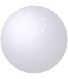
The metric topology of a metric space is built atop the basis set of that metric space. In particular, for any family of open sets $\mathcal{B}$ of metric space $(X,d)$, $\mathcal{B}$ is a basis set if every open subset of $(X,d)$ is a union of sets in $\mathcal{B}$
A topology has three axioms which define both how to build them and how they behave, see Eq. $\eqref{axiom:topo-1}$, $\eqref{axiom:topo-2}$, $\eqref{axiom:topo-3}$, see
Proposition 1.
There exists a topological basis $\mathcal{B}$ for metric topology $\mathcal{T}$ formed from the metric space $(\widehat{\mathbb{C}}, d_{ch})$
Proof of Proposition 1
Recall that $(\widehat{\mathbb{C}}, d_{ch})$ is a metric space
Open sets in a metric space have the form $B(x; \epsilon)$

Lemma 1
The set $\mathcal{B}$ has the intersectional property.
Proof of Lemma 1
The open sets $U, V \in \mathcal{B}$ must be open balls, thus let us define them as Eq. $\eqref{def:u-v}$. \(\begin{equation} \label{def:u-v} \begin{split} U := B(a ; r_U) \\ V := B(b ; r_V) \end{split} \end{equation}\)
Such that some point $z$ has the property $z \in B(a ; r_U) \cap B(b ; r_V)$. Given that $U \cap V \ne \emptyset$ we can say that there exists $W \in U \cap V$. In particular, we can describe $W$ as that open ball centered on the point $z$ with radius of the shortest distance to the bound of either intersecting set Eq. $\eqref{def:w1}$.
\[\begin{equation} \label{def:w1} \begin{split} W := B(z ; r_W) \\ r_W = min[(r_U - d(z,a)),(r_V - d(z, b))] \end{split} \end{equation}\]This grantees the relationship $W \subseteq U \cap V$ which is not quite the desired $W \subset U \cap V$, the fix is observed by Eq. $\eqref{def:w2}$.
\[\begin{equation} \label{def:w2} \begin{split} W := B(z ; r_W) \\ r_W = \frac{1}{2}min[(r_U - d(z,a)),(r_V - d(z, b))] \end{split} \end{equation}\]This guarantees the desired relation $z \in W \subset U \cap V$ required by the intersection property. The remaining doubt is that all elements of $W$ belong to both $U$ and $V$. This can easily be observed through the triangle inequality. It is observed that for any point $w \in W$ that $d(a,w) \le d(a,z) + d(z,w) < d(z,a) + r_W < r_U$. The same relation is observed for $V$, therefore all elements of $W$ belong to $U$ and $V$.
Given the above information on $\mathcal{B}$ and Lemma 1 it proved a basis set. Therefore the metric topology $\mathcal{T}$ exists and takes the form of Eq. $\eqref{def:T-from-basis}$.
Compactness of \(\widehat{\mathbb{C}}\)
A space is said to be compact if every open cover of that space has a finite subcover
Proposition 2
$\widehat{\mathbb{C}}$ is a compactification of $\mathbb{C}$.
Proof of Proposition 2
First let us prove that $\mathbb{C}$ is not compact.
Lemma 1
$\mathbb{C}$ is not compact.
Proof of Lemma 1
Any compact set must be closed and bounded
Lemma 2
There exists a homeomorphism $f: \widehat{\mathbb{C}} \rightarrow S^2$ such that $\widehat{\mathbb{C}}$ and $S^2$ are homeomorphic.
Proof of Lemma 2
Recall that in
It can now understood by Lemma 2 that if $S^2$ is shown to be compact then so is $\widehat{\mathbb{C}}$ via the laws of topology
Lemma 3
$S^2$ is compact via the Hiene-Borel theorem Eq. $\eqref{def:HB}$.
Proof of Lemma 3
The set $S^2$ defined by Eq. $\eqref{def:S2}$ is obviously a bounded subset of $\mathbb{R}^3$.
\[\begin{equation} \label{def:S2} S^2 := \{ x : (x \in \mathbb{R}^3) \land (\|x\| = 1) \} \end{equation}\]There exists a continuous function $f$ defined by Eq. $\eqref{def:f}$ such that $f$ is continuous.
\[\begin{equation} \label{def:f} \begin{split} f &: \mathbb{R}^3 \rightarrow \mathbb{R} \\ f(x) &= \| x \| \end{split} \end{equation}\]Notably the pre-image of a closed set is closed via a continuous function across two metric spaces
It has been proven that $S^2$ is both bounded and closed in $\mathbb{R}^3$, proving by Eq. $\eqref{def:HB}$ that $S^2$ is compact.
Given Lemma 1, Lemma 2 & Lemma 3 it can be said that $\widehat{\mathbb{C}}$ is a compactification of $\mathbb{C}$.
Dense subsequence
It is worth exploring a specific dense subset of $\widehat{\mathbb{C}}$ as it will be of importance. Let us define the set $\Omega$ as those points rational points of $\widehat{\mathbb{C}}$ including the point $\infty$. In particular it can be seen by Eq. $\eqref{def:omega}$ that $\Omega \subset \widehat{\mathbb{C}}$, as the complex numbers are isomorphic to $\mathbb{R}^2$ not $\mathbb{Q}^2$.
\[\begin{equation} \label{def:omega} \begin{split} \Omega := (\mathbb{Q} + i\mathbb{Q} \cup \{ \infty \}) \subset \widehat{\mathbb{C}} \end{split} \end{equation}\]Proposition 3
$\Omega$ is dense in $\widehat{\mathbb{C}}$.
Proof of Proposition 3
A dense subset is defined as that subset $U$ of a space $X$ for which the closure of the subset $\bar{U}$ is the space Eq. $\eqref{def:dense-subset}$.
\[\begin{equation} \label{def:dense-subset} U \text{ dense in } X \implies \bar{U} = X \end{equation}\]The closure of the rational numbers is the real numbers $\bar{\mathbb{Q}} = \mathbb{R}$ implies that $\overline{\mathbb{Q} + i\mathbb{Q}} = \mathbb{R} + i\mathbb{R}$. Thus it must be true that \(\mathbb{Q} + i\mathbb{Q} \cup \{ \infty \}\) is dense in \(\mathbb{R} + i\mathbb{R} \cup \{ \infty \}\), proving that $\Omega$ is dense in $\widehat{\mathbb{C}}$.
Computability
A computable process can be defined as that mechanical logic which accomplishes a decidable predicate in finitely many steps
It is understood that $\mathbb{R}^2$ is isomorphic to $\mathbb{C}$ and $\widehat{\mathbb{C}}$ is isomorphic to $S^2$, therefore a region in our sense will be that open connected subset of $\widehat{\mathbb{C}}$.
Classical approach
To examine the computability of any region of $\widehat{\mathbb{C}}$ it is imperative to understand what it means for a set to be computable or recursive. Formally we say that a set is recursive when its characteristic function is computable
It is clear that a set is recursive only when its characteristic function is computable, thus possessing a decidable predicate $x \in A$. Via
Computable topologies
Having deduced that classical computability does not have the power to examine the computability of $\widehat{\mathbb{C}}$ presenting an opportunity to examine modern approaches. The space of computability I investigate here is that of metric spaces on $\mathbb{R}^n$ where $(n \ge 1)$. There exists a literature for computability on metric spaces belonging to $\mathbb{R}^n$
- $(M,d)$ is a metric space
- $A \subset M$ is dense in $M$
- $\alpha : \mathbb{N} \rightarrow A$ is a total numbering of $A$
- \(D_{<} := \{ \langle i, j, k \rangle \mid d(\alpha(i), \alpha(j)) < v_\mathbb{Q}(k) \}\) is recursively enumerable
Therefore by TTE if one can satisfy and prove the validity of the four elements of the tuple $\bar{M}$ then one proves the effectivity of the space $(M, d)$. In the article so far It is clear that the metric space under investigation is $(\widehat{\mathbb{C}}, d_{ch})$. Notably it was proven that $\Omega$ from Eq. $\eqref{def:omega}$ is a dense subset of this metric space. Thus if there exists functions $\alpha$ and $D_{<}$ then the existence of recursively enumerable regions or $(\widehat{\mathbb{C}}, d_{ch})$ can be proved to exist.
Proposition 4
There exists a tuple $\bar{M}$ of the form described by equation Eq. $\eqref{construct:bar-M}$ that satisfies TTE.
\(\begin{equation} \label{construct:bar-M} \bar{M} := ((\widehat{\mathbb{C}}, d_{ch}), \Omega, \alpha, D_<) \end{equation}\)
Proof of Proposition 4
It is clear from proposition 3 that $Omega$ is dense in $\widehat{\mathbb{C}}$ there for it suffices to show the existence and definition of both $\alpha$ and $D_<$.
Lemma 1
There exists a bijection $\alpha$ of the form $\mathbb{N} \mapsto \Omega$.
Proof of Lemma 1
It is clear that $\Omega$ is isomorphic to that of $\mathbb{Q}^2$, therefore it suffices to show that $\mathbb{Q}^2$ is denumerable. In particular, It must be shown that a bijection $\alpha: \mathbb{N}^2 \rightarrow \mathbb{Q}^2$ exists. It is a standard fact of analysis that $\mathbb{Q}$ is denumerable. Notably the Cartesian product of any two denumerable sets is its denumerable
The function $v_\mathbb{Q}$ is that most natural mapping $\mathbb{N} \mapsto \mathbb{Q}$. Therefore $D_<$ can be described as those the set of natural three tuples for which the $d_{ch}(\alpha(i), \alpha(j)) < v_\mathbb{Q}(k)$. From Lemma 1 it is clear that alpha will result in elements of $\Omega$, using the chordal metric $d_{ch}$ results in some distance $z \in \mathbb{C}$. Therefore the set $D_<$ is all those natural three tuples which result in a complex distance on $\widehat{\mathbb{C}}$ which is less than some rational mapping $v_\mathbb{Q}(k)$.
Lemma 2
The set $D_<$ is recursively enumerable.
Proof of Lemma 2
The set $D_<$ defined by Eq. $\eqref{def:D<}$ is that set composed of natural triples satisfying the condition $d_{ch}(\alpha(i), \alpha(j)) < v_\mathbb{Q}$.
\[\begin{equation} \label{def:D<} D_< := \{\langle i, j ,k \rangle : d_{ch}(\alpha(i), \alpha(j)) < v_\mathbb{Q}(k) \} \end{equation}\]To prove a set $A$ is recursively enumerable one must show there exists a partially decidable predicate $x \in A$. In particular one must prove that some characteristic function $c_A$ exists defined as Eq. $\eqref{def:c_A}$
Notably that predicate defining ownership to a set must be decidable while that predicate of non ownership is undecidable. This means that Lemma 2 sets out to prove $\langle i, j, k \rangle \in D_<$ is decidable. To this end the condition described above must be further investigated. The chordal metric $d_{ch}$ is defined as Eq. $\eqref{def:dch}$ via
It is clear that given $\alpha: \mathbb{N} \rightarrow \Omega$ we can track the result number ring of the image of $d_{ch}$. It is trivial to see that $d_{ch}$ given points from $\Omega$ results in numbers from $\mathbb{R}$. The objective is then to show that there exists an algorithm which can show the real number resulting from $d_{ch}(\alpha(i), \alpha(j))$ is less that $v_\mathbb{Q}(\alpha(k))$. Therefore the set $D_<$ has the characteristic function $c_{D_<}$ defined in Eq. $\eqref{def:c-D<}$.
\[\begin{equation} \label{def:c-D<} c_{D_<} = \begin{cases} 1, \quad &\langle i, j, k \rangle \in D_< \\ \text{undefined}, \quad &\langle i, j, k \rangle \notin D_< \end{cases} \end{equation}\]The algorithm that proves the decidability of $\langle i, j, k \rangle \in D_<$ is defined by Eq. $\eqref{def:pred-D<}$ for both cases of $d_{ch}$ (non-infinite and infinite).
\[\begin{equation} \label{def:pred-D<} \begin{split} \langle i, j, k \rangle \in D_< &\iff d_{ch}(\alpha(i), \alpha(j)) < v_\mathbb{Q}(k) \\ d_{ch}(\alpha(i), \alpha(j)) &:= \frac{2|\alpha(i) - \alpha(j)|} {\sqrt{(1 + |\alpha(i)|^2)(1 + |\alpha(j)|^2)}} \\ d_{ch}(\alpha(i), \infty) &:= \frac{2}{\sqrt{1 + |\alpha(i)|^2}} \end{split} \end{equation}\]Concerning the predicate shown in Eq. $\eqref{def:pred-D<}$ it suffices to show that an algorithm exists that can construct the set $D_<$. One such algorithm would be to iterate through all the natural numbers including infinity and include the resulting element in $D_<$ depending on the condition.
function cond(i, j, k) {
    if d_ch(alpha(i), alpha(j)) < v_Q(alpha(k))
        return (i, j, k)
    return None
}

function main() {
    for i, j, k \in (\N union \infty){
        if cond(i, j, k) != None
            D_<.append(cond(i,j,k))
    }
}
The code snippet above presents an algorithm constructing the potentially infinite set $D_<$. Let alpha be the $\alpha$ function; let \N represent the natural numbers; finally let \infty represent infinity as a point \(\{ \infty \}\). Notably this construction is not optimal though it does prove to show that such a construction is describable using the standard mechanistic logic (C-style pseudocode). Therefore the valid triples belonging to $D_<$ can be found via an $n^3$ algorithm searching all combinations of numbers and checking the condition of Eq. $\eqref{def:pred-D<}$.
By the above $D_<$ is proved to be recursively enumerable.
With the addition of Lemma 2 it has been proven that there exists a tuple $\bar{M}$ satisfying TTE.
Future work
This kind of investigation is quite rewarding though extensions of this work seem substantial comparatively. One could postulate the construction of such a computable region using research in computable geometry. There is a possibility that such an exercise could be useful in furthering understanding $\widehat{\mathbb{C}}$ topologically. In particular in the sense that computational geometry could construct such a region of $\widehat{\mathbb{C}}$ without interpolation or approximation. I would personally love to see such a construction. The extensions of the use case for TTE are endless, moving forward it will be inevitable to halt curiosity in using the tool to examine such structures.
Nomenclature
- $\emptyset$: Symbol for the empty set \(\{\}\).
- $\subset$: Symbol for subset.
- $\widehat{\mathbb{C}}$: Symbol for the Riemann sphere.
- $x \in A$: $x$ is an element of the set $A$.
- \(\{ x: (x \in A) \land (x > 0)\}\): set builder notation, read: all elements $x$ such that $x \in A$ logical and $x > 0$.
- $S^2$: The unit sphere projected in $\mathbb{R}^3$.
- $\exists x$: There “exists” some value $x$
- $v_\mathbb{Q}: \mathbb{N} \rightarrow \mathbb{Q}$: the standard numbering on $\mathbb{Q}$ inherited from
. - $\mathbb{B}$: Baire space notation inherited from
. - $x \notin A$: The element $x$ can not be found in the set $A$.
- $\bar{U}$: denoting the closure of set $U \subseteq X$ in the space $X$.