Computable regions of the Riemann sphere

Exploring computability in the context of the Riemann sphere

Introduction

I examine the Riemann sphere in terms of its computability. In particular does there exist those regions of $\widehat{\mathbb{C}}$ that can be proven recursive and how? To this end I find myself examining how computability is defined on analytic structures. Which structures can be explored in terms of recursion theory, and if they can be explored how? It is precisely these questions that I explore in the article. In the pursuit of the above queries an exploration of topology seemed enjoyable and necessary. Once the topology of $\widehat{\mathbb{C}}$ is described shallowly, the article shifts to finding a suitable theory of recursion for a possible proof.

Topology of Riemann sphere

Here I discuss the topology $\widehat{\mathbb{C}}$ defined by \(\mathbb{C}_\infty\) and the chordal metric $d$ (stereographic projection) described in . That is the topology $\mathcal{T} := (\widehat{\mathbb{C}}, d)$. All topologies must adhere to the axiomatic definition of a topology . For any set $X$, the topology $\mathcal{T}$ has the following properties:

$ \begin{equation} \label{axiom:topo-1} X, \emptyset \in \mathcal{T} \end{equation} $

$ \begin{equation} \label{axiom:topo-2} (A, B \in \mathcal{T}) \implies (A \cup B \in \mathcal{T}) \end{equation} $

$ \begin{equation} \label{axiom:topo-3} (n \in \mathbb{N} \land n \ne \infty), \cap_{j<n} \mathcal{T}_j \in \mathcal{T} \end{equation} $

A metric topology is defined such that every open set corresponds to an open ball. An open ball is defined by can be seen in Eq. $\eqref{eq:open-ball}$.

$ \begin{equation} \label{eq:open-ball} B(x; r) = {y \in X: d(x,y) < r} \end{equation} $

In particular it is the set created when given some point $x$ all points $y$ are defined by the radius $r$. Those points $y$ are within the distance $r$ defined by the metric function $d$ of $x$. It is important to note that those points at exactly distance $r$ are excluded from the set. The topology investigated here is the metric topology where all open sets are defined by the open ball Eq. $\eqref{eq:open-ball}$.

Proposition 1.

$\mathcal{T} := (\widehat{\mathbb{C}}, d)$ forms a metric topology over $\widehat{\mathbb{C}}$.

Proof.

Note the construction of $\mathcal{T}$ is described by Eq. $\eqref{eq:topo-construction}$.

\[\begin{equation} \label{eq:topo-construction} \mathcal{T} := \{ B(x;\epsilon): x \in \widehat{\mathbb{C}}, \epsilon > 0 \} \end{equation}\]

If $\mathcal{T}$ is the topological set of all open balls in $(\widehat{\mathbb{C}}, d)$, then there exists a basis $\mathcal{B}$ by which we can prove $\mathcal{T}$ is a topology. That is the family of open sets $\mathcal{B}$ has the following property.

\[\begin{equation} \label{eq:basis-neighborhoods} \begin{split} \mathcal{B} &\subset \mathcal{T} \\ (\forall B \in \mathcal{B})(x \in B) &\implies (\exists V: x \in V) \end{split} \end{equation}\]

The set $\mathcal{T}$ is the set of all open balls, thus for each $x \in \widehat{\mathbb{C}}$ we have that there exists $x \in B(x;r) \subset \mathcal{B}$. That is there exists an open ball centered on every element of the Riemann sphere. According to any basis of a topology must have the following property.

\[\begin{align} \bigcup \mathcal{B} &\subset X \\ \label{prop:elem-in-B} (x \in X) &\implies (\exists B(x;\epsilon) \subset \mathcal{B}: \epsilon > 0) \\ \label{prop:intersection-W} (U,V \in \mathcal{B}) \land (x \in (U \cap V)) &\implies (\exists W \in \mathcal{B}) \land (x \in W \subset (U \cap V)) \end{align}\]

Thus proving that the basis $\mathcal{B}$ described for $\mathcal{T}$ has the qualities described above. By the construction of $\mathcal{T}$ we know that all elements $x \in \widehat{\mathbb{C}}$ have an open ball centered on them, satisfying property $\eqref{prop:elem-in-B}$. That is there exists a family open sets $\mathcal{B} \subset \mathcal{T}$ for which all elements of the space are contained in those open sets. By the construction of $\mathcal{T}$, all open balls defined by the metric space $(\widehat{\mathbb{C}}, d)$. Assume for a contradiction that property $\eqref{prop:intersection-W}$ is not true for $\mathcal{T}$. This means that there is no such basis for which the interaction of any two non-disjoint open balls contains a second open ball. By the construction of $\mathcal{T}$ it is not only possible but defined that each element is contained in an open ball of size one. That is if we have two non-disjoint open balls $B$ and $V$ such that there intersection is not empty then by definition there must exist an open ball in their intersection, a contradiction This proof is remarkably fun to visualize. .

Figure 1: Intersection property of topological basis sets

Now that I have crafted a somewhat convincing argument for the existence of a topology on $(\widehat{\mathbb{C}}, d)$ let us analyze it.

A metric topology such as $\mathcal{T}$ is defined by its open sets, recall the basis is a family of open sets. Open sets are defined in a metric topology as those sets centered on an element $x$. In particular, those sets for which every element of the sets is within some distance $\epsilon$ from $x$ using the metric function $d$. Recall $d$ is defined in as \(d(z, z') = [(x_1 - x'_1)^2+(x_2-x'_2)^2+(x_3-x'_3)^2]^\frac{1}{2}\), the euclidean distance between two points in $\mathbb{R}^3$. Thus for any point $z \in \widehat{\mathbb{C}}$, it is trivial to see that the open set $B(z; \epsilon)$ is defined as ${x: d(z,x) < \epsilon} $. That is each open ball includes all those points within some distance from $x$. On a plane this presents as a circle where that distance acts as the radius. On $S^2$ that is the projection of plane in $\mathbb{R}^3$ as a sphere an open ball would be visualized as a circle. Seeing as $S^2$ is homeomorphic to $\widehat{\mathbb{C}}$ (see the construction in ) it becomes tempting to believe open balls appear the same on $\widehat{\mathbb{C}}$ as $S^2$. Recall that $\infty$ is a point on $\widehat{\mathbb{C}}$ a point of infinite distance. Noticeably those points closest to the north-pole still have the property $d(N, z) = \infty$. This property is most clearly observed through a visualization of an open ball with a finite $\epsilon$ value.

Figure 2: Visualization of open set on Riemann sphere

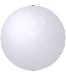
Figure 2 gives an exaggerated concept of the effects of infinity at the north pole. Open balls constructed with a finite distance will always have a concavity surrounding the point infinity. The distance from zero will cascade along the south to north poles creating rings of equivalent distance from zero. This idea is shown by Figure 3, by visualizing all the elements at three different, constant, finite distances from zero shown by red rings. That is no finite point $z$ is ever closer to the point infinity than $d(z, \infty) = \infty$ .

Figure 3: visualization of equivalently distant elements from zero

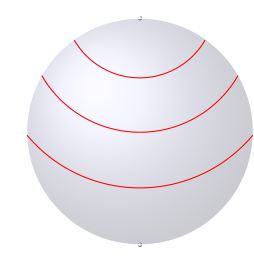
We can see three different open balls in Figure 3, all centered on the zero point or the south pole. In particular we have three open balls such that $B’’ \subset B’ \subset B$, where the distance value of each open ball is greater than the last. Thus it is possible to observe one of the axioms of topology \(\widehat{\mathbb{C}} \subset B(0; \infty) \in \mathcal{B} \subset \mathcal{T}\) . This concept nicely leads into the observation of closed sets present in $\mathcal{T}$. The definition of a closed set I focus on here is that a set is closed iff its compliment set is open . Thus by the pictures above closed sets would encompass all those points not contained in the open balls (including the open balls boundaries). In particular, it is usual to call these sets closed balls \(\bar{B}(z; \epsilon) = \{x: (d(z, x) \le \epsilon) \land (\epsilon > 0)\}\). As a final note I would assert that not all open and closed sets are as uniform as the above visualizations make them seem, it is simply easier to demonstrate with smooth uniform sets.

The second important topological examination needed for the article is that of compact sets. A set is compact if every open cover of it has a finite subcover . Intuitively that is for ever family of open sets \(\{U_\alpha\}_{\alpha \in A}\) the union of that family is the topological space \(\bigcup \{U_\alpha\}_{\alpha \in A} = X\). Presented more formally in Eq. $\eqref{prop:compact-def}$ we see that intuitively a set is compact iff any open cover of that set has only finitely many open sets .

\[\begin{equation} \label{prop:compact-def} \begin{split} (U := {U_\alpha}_{\alpha \in A}) &\land (\bigcup U_\alpha = X) \\ \text{X is compact } &\iff A \ne \infty \end{split} \end{equation}\]

It is trivial to see that $\mathbb{C}$ is not compact by intuiting this geometrically. Visualizing $\mathbb{C}$ as a plane it is impossible to see the edge of such a plane. In particular, it is impossible intuitively for a finite amount of open sets to cover such a plane. Noticeably this intuition provides us with the inference that if a set is not self contained then its probably not compact. Formally this statement is thus: a set is compact iff it is closed and bounded . In particular, a closed set contains its limit points and a bounded set has some bounding. It may now be asked if indeed the Riemann sphere is compact. Noticeably $\widehat{\mathbb{C}}$ is that extension of $\mathbb{C}$ containing the point $\infty$. In the intuition of $\mathbb{C}$ it was simple to use the geometry to imagine if some amount of sets could cover the plane. Geometrically $\widehat{\mathbb{C}}$ is not presented as a plane, it is presented via that homeomorphism of $S^2$ . The Riemann sphere is projected into $\mathbb{R}^3$ via stereographic projection, though it is essentially still a plane with a single point of convergence. This can be intuited by the hollowness of the Riemann sphere, that is only the points on the surface of the sphere are technically contained in $\widehat{\mathbb{C}}$. All of this is to say the geometric version of this proof would be bothersome. Luckily the Heine-Borel theorem states: A subset $K$ of $\mathbb{R}^n, (n ge 1)$ is compact iff $K$ is closed and bounded. Unfortunately $\widehat{\mathbb{C}}$ is an extension of $\mathbb{C}$ which is not contained by $\mathbb{R}$, this is not true of $S^2$.

Proposition 2.

The Riemann sphere $\widehat{\mathbb{C}}$ is a compactification of $\mathbb{C}$.

Proof

Recall the Heine-Borel theorem.

\[\begin{aligned} \label{theorem:h-b} (X \subset \mathbb{R}^n) &\land (n \ge 1) \\ (\exists sup(X) < \infty) &\land (\exists inf(X) > -\infty) \\ \end{aligned}\]

In particular, the Heine-Borel dictates that the space must have a finite supremum and infimum. The unit sphere $S^2$ is bounded by this definition as it possess both a finite supremum and infimum in $\mathbb{R}^3$. It is also the case that $S^2 \subset \mathbb{R}^3$ by definition of $S^2$. Therefore $S^2$ is compact by the Heine-Borel theorem. Noticeably $\widehat{\mathbb{C}}$ is constructed via stereographic projection from $S^2$. As the definition of a homeomorphism is some bijection between two space s, $\widehat{\mathbb{C}}$ and $S^2$ are homeomorphic by definition. It is also the case that homeomorphisms serve as topological equivalence relations between spaces . Therefore if $S^2$ is compact and homeomorphic to $\widehat{\mathbb{C}}$ implies that $\widehat{\mathbb{C}}$ is compact I love this proof, however it does make me nervous due to its shortness .

Computability

A computable process is usually defined as that mechanical logic which accomplishes some decidable predicate in finitely many steps . In particular, the idea of computability is heavily dependant on the logic in use. Let the definition of decidability be adopted from , as a full treatment is beyond the scope of this article. Here I will use the idea of Turing-computability, though my understanding of such mechanical logic is more closely tied to the Lambda calculus. In particular this means that here a computable function utilizes the Turing machine as a mechanical logic. We first examine the use of classical computability applied to the problem, then examine some more modern methodology.

Classical approach

To examine the computability of any region of $\widehat{\mathbb{C}}$ it is imperative to understand what it means for a set to be computable. First it is said that a set is recursive when its characteristic function is computable . Moving forward note that this article will use the term recursive when discussing sets, and computable when discussing functions. A sets characteristic function is the ownership defining function corresponding to the predicate $x \in A$. Formally for any set $A$ the characteristic function $c_A: \mathbb{N} \rightarrow A$ is that function which computes $x \in A$. Notably $c_A$ shown in Eq. $\eqref{fxn:c_A}$ is computable iff $x \in A$ is a decidable predicate.

\[\begin{equation} \label{fxn:c_A} c_A = \begin{cases} 1 \quad \text{if } x \in A \\ 0 \quad \text{if } x \notin A \\ \end{cases} \end{equation}\]

It is clear that a set is recursive only when its characteristic function is computable, thus possessing a decidable predicate $x \in A$. Via all characteristic functions (recursive sets) are defined with denumerable domains (domains mappable to $\mathbb{N}$), as the sets themselves must be denumerable. In particular, it is the case that in classical computability recursive sets are defined to be natural or natural adjacent . Notably classical computability via has no power over $\widehat{\mathbb{C}}$. This result implies that it is an impossibility to use classical recursion theory to investigate $\widehat{\mathbb{C}}$.

Computable topologies

Having deduced that classical computability does not have the power to examine the computability of $\widehat{\mathbb{C}}$ we turn to modern approaches. The space of computability I investigate here is that of metric spaces under $\mathbb{R}^n$. There exists a literature for computability on metric spaces belonging to $\mathbb{R}^n$ . The literature describes the “classical approach” above as type one theory of computability. As discussed the type one theory is ineffective on spaces on the order of $\mathbb{R}^n$ where $n \ge 1$. The literature then converges on which describes the type two theory of computability (TTE) which works in spaces on the order of $\mathbb{R}^n$. The TTE has only appeared so far in writings stemming from in my readings. There exist previous sources of computability on broader spaces than $\mathbb{N}$ though none as general as TTE. Notably TTE claims power enough to prove $\mathbb{R}$ a computable space . For the scope of $\widehat{\mathbb{C}}$ TTE provides insight into computability of metric spaces. Such that TTE describes a theory of computability tied to specific topologies known as Baire spaces . TTE describes a computable metric space as the four tuple $\bar{M}$ described in Eq. $\eqref{eq:tte-m}$. Dictating that the cardinality of $M$ be at most that of a Baire space, $card(M) \le card(\mathbb{B})$.

\[\begin{equation} \label{eq:tte-m} \bar{M} := (M, d, A, \alpha) \end{equation}\]

1. $(M,d)$ is a metric space
2. $A \subset M$ is dense in $M$
3. $\alpha : \mathbb{N} \rightarrow A$ is a total numbering of $A$
4. $D_{<} := { \langle i, j, k \rangle \mid d(\alpha(i), \alpha(j)) < v_\mathbb{Q}(k) }$ is recursively enumerable

Intuitively if $\mathbb{R}$ is computable via TTE then so should be $\mathbb{C}$. The key to a proof seems to be finding a dense, denumerable subset of $\mathbb{C}$. I have selfishly stopped myself from searching the literature for such a set, as my intuition tells me that one exists. If such a set exists for $\mathbb{C}$ one could conceivably build a proof intuitively given a partial order is chosen. It is much more difficult to imagine a proof of $\widehat{\mathbb{C}}$ as a dense set would need to include $\infty$ as a limit point while still being denumerable.

Future work

I would love to dedicate a full length article to the proof of computability of $\widehat{\mathbb{C}}$ via TTE. There is a fair amount of work in the area of topological computability by Brattka and Weihrauch that I intend to consume. The field itself is very interesting especially paired with Conway’s texts on complex analysis. Alas my number theory, topology, and analysis are all just a bit too under developed to move further at this time.

Nomenclature

1. $\emptyset$: Symbol for the empty set \(\{\}\).
2. $\subset$: Symbol for subset.
3. $\widehat{\mathbb{C}}$: Symbol for the Riemann sphere.
4. $x \in A$: $x$ is an element of the set $A$.
5. \(\{ x: (x \in A) \land (x > 0)\}\): set builder notation, read: all elements $x$ such that $x \in A$ logical and $x > 0$.
6. $S^2$: The unit sphere projected in $\mathbb{R}^3$.
7. $\exists x$: There “exists” some value $x$
8. $v_\mathbb{Q}: \mathbb{N} \rightarrow \mathbb{Q}$: the standard numbering on $\mathbb{Q}$ inherited from .
9. $\mathbb{B}$: Baire space notation inherited from .